Discover and Visualize the Data to Gain Insights on Feature vs Label Correlations: OkCupid Dataset

Identifying Correlations

Refining Offspring Categories for Clarity in Analysis

We first need to merge some classes of features into broader classes. That way, we can better capture the big picture in the plots we generate.

./chapter2/data2/load3.py

import os
import pandas as pd

DATING_PATH = os.path.join("datasets", "dating")

def load_dating_data(dating_path=DATING_PATH):
    csv_path = os.path.join(dating_path, "male_straight_data_with_classified_columns.csv")
    return pd.read_csv(csv_path)

dating_data = load_dating_data()

print(f"\nTotal entries in the dataset: {len(dating_data)}")


target_columns = ['status', 'offspring']

print("\nValue counts for specified columns:")
for column in target_columns:
    if column in dating_data.columns:
        print(f"\n{column} value counts:")
        print(dating_data[column].value_counts(dropna=False))
    else:
        print(f"\nWarning: {column} not found in the dataset.")


print(f"\nTotal entries in the dataset: {len(dating_data)}")

print("\nNumber of non-missing rows per column:")
for column in dating_data.columns:
    non_missing_count = dating_data[column].notna().sum()
    print(f"{column}: {non_missing_count} non-missing rows")

Classifying Offspring: Applying Consistent Rules

Below are the possible values for "offspring":

offspring value counts:
offspring
NaN                                        18927
doesn't have kids                           4192
doesn't have kids, but might want them      2128
doesn't have kids, but wants them           1622
doesn't want kids                           1228
has kids                                     912
has a kid                                    835
doesn't have kids, and doesn't want any      519
has kids, but doesn't want more              180
has a kid, and might want more               139
might want kids                               98
has a kid, but doesn't want more              93
wants kids                                    77
has kids, and might want more                 67
has a kid, and wants more                     44
has kids, and wants more                      12
Name: count, dtype: int64

We need to classify offspring based on specific rules.

We use this classification map to classify all possible entry values for offspring:

The logic is that 0 is assigned to people with no children, 1 is assigned to people with one kid, and 2 is assigned to people with at least two kids.

classification_map = {
    "doesn't have kids": 0,
    "doesn't have kids, but might want them": 0,
    "doesn't have kids, but wants them": 0,
    "doesn't want kids": 0,
    "doesn't have kids, and doesn't want any": 0,
    "might want kids": 0,
    "wants kids": 0,
    "has a kid": 1,
    "has a kid, and might want more": 1,
    "has a kid, but doesn't want more": 1,
    "has a kid, and wants more": 1,
    "has kids": 2,
    "has kids, but doesn't want more": 2,
    "has kids, and might want more": 2,
    "has kids, and wants more": 2,
}

We execute the code below to generate the new column that broadens the categories. This permits us to have a lower number of groups in total. The new groups are sufficiently distinctive from one another, so the loss in terms of specificity is not as lost:

./chapter2/data2/data_manipulations2/step6.py

import os
import pandas as pd

# Define the path to the dataset folder
DATING_PATH = os.path.join("datasets", "dating/copies2")

# Function to load the dataset (male-only, straight)
def load_dating_data(dating_path=DATING_PATH):
    csv_path = os.path.join(dating_path, "copy1_male_straight_data_with_classified_columns.csv")
    return pd.read_csv(csv_path)

# Function to classify offspring based on your provided rules
def classify_offspring(offspring):
    if pd.isna(offspring):
        return float('nan')  # Keep NaN as is

    # Mapping specific offspring values to corresponding classifications
    classification_map = {
        "doesn't have kids": 0,
        "doesn't have kids, but might want them": 0,
        "doesn't have kids, but wants them": 0,
        "doesn't want kids": 0,
        "doesn't have kids, and doesn't want any": 0,
        "might want kids": 0,
        "wants kids": 0,
        "has a kid": 1,
        "has a kid, and might want more": 1,
        "has a kid, but doesn't want more": 1,
        "has a kid, and wants more": 1,
        "has kids": 2,
        "has kids, but doesn't want more": 2,
        "has kids, and might want more": 2,
        "has kids, and wants more": 2,
    }

    # Standardizing the input string to match the keys in the map
    offspring = offspring.strip().lower()
    
    # Return the corresponding classification or NaN if not found
    return classification_map.get(offspring, float('nan'))

# Load the dataset
male_data = load_dating_data()

# Apply the offspring classification and add it as a new column
male_data['classified_offspring'] = male_data['offspring'].apply(classify_offspring)

# Save the updated dataset with the new column
output_path = os.path.join(DATING_PATH, "copy2_male_straight_data_with_classified_columns_classify_offspring.csv")

male_data.to_csv(output_path, index=False)

print(f"Dataset with classified offspring saved to: {output_path}")

Classifying Relationship Status for Better Insights

We now need to classify "status", and these are the possible values for "status":

status value counts:
status
single            29163
available           899
seeing someone      854
married             152
unknown               5
Name: count, dtype: int64

We use this classification map to classify all possible entry values for status based on specific rules.

The logic is that 0 is assigned to singles. 1 is assigned to people with a status of 'available.' The status 'available' implies not being single and being open to mating options.

'Seeing someone' and 'married' both mean that someone is consistently engaging with a partner; therefore, a label of 2 will be assigned.

classification_map = {
    "single": 0,
    "available": 1,
    "seeing someone": 2,
    "married": 2,
    "unknown": float('nan')  # Handle unknown cases as NaN
}

Transforming Relationship Status into Categorical Values

We execute the code below to generate the new column of numbered statuses:

./chapter2/data2/data_manipulations2/step7.py

import os
import pandas as pd

# Define the path to the dataset folder
DATING_PATH = os.path.join("datasets", "dating/copies2")

# Function to load the dataset (male-only, straight)
def load_dating_data(dating_path=DATING_PATH):
    csv_path = os.path.join(dating_path, "copy2_male_straight_data_with_classified_columns_classify_offspring.csv")
    return pd.read_csv(csv_path)

# Function to classify status based on the provided mapping
def classify_status(status):
    if pd.isna(status):
        return float('nan')  # Keep NaN as is

    # Mapping specific status values to corresponding classifications
    classification_map = {
        "single": 0,
        "available": 1,
        "seeing someone": 2,
        "married": 2,
        "unknown": float('nan')  # Handle unknown cases as NaN
    }

    # Standardizing the input string to match the keys in the map
    status = status.strip().lower()
    
    # Return the corresponding classification or NaN if not found
    return classification_map.get(status, float('nan'))

# Load the dataset
male_data = load_dating_data()

# Apply the status classification and add it as a new column
male_data['classified_status'] = male_data['status'].apply(classify_status)

# Save the updated dataset with the new column
output_path = os.path.join(DATING_PATH,"copy3_male_straight_data_with_classified_columns_classify_offspring_classified_status.csv")
male_data.to_csv(output_path, index=False)

print(f"Dataset with classified status saved to: {output_path}")

Investigating Key Feature Correlations with Mating Success

We study the correlations of the label (mating_success) vs other features (age, classified_ethnicity, height, income, classified_body_type, classified_drinks, classified_smokes, classified_drugs, classified_religion, classified_speaks) to understand the data we have.

The label is called 'mating_success' and scales from 0 to 6.

The label is computed based on the value of the entries' offspring' and 'status' features. These features are crucial in understanding the individual's family and relationship status, which can significantly influence their mating success.

Below is the code used to compute the label's (mating_success) value:

./chapter2/data2/data_manipulations2/step8_1.py

import os
import pandas as pd

# Define the path to the dataset folder
DATING_PATH = os.path.join("datasets", "dating/copies2")

# Function to load the dataset (male-only, straight)
def load_dating_data(dating_path=DATING_PATH):
    csv_path = os.path.join(dating_path, "copy3_male_straight_data_with_classified_columns_classify_offspring_classified_status.csv")
    return pd.read_csv(csv_path)

# Function to compute mating_success based on the specified logic
def compute_mating_success(row):
    status = row['classified_status']
    offspring = row['classified_offspring']

    # Handle cases based on the new logic
    if pd.isna(status) and pd.isna(offspring):
        return float('nan')
    elif pd.isna(status) and not pd.isna(offspring):
        return offspring * 2
    elif not pd.isna(status) and pd.isna(offspring):
        if status == 0:
            return float('nan')  # status is 0 -> mating_success is NaN
        elif status == 1:
            return 1  # status is 1 -> mating_success is 1
        elif status == 2:
            return 2  # status is 2 -> mating_success is 2
    else:
        # If both status and offspring are present
        return status + offspring * 2

# Load the dataset
male_data = load_dating_data()

# Apply the function to calculate mating_success
male_data['mating_success'] = male_data.apply(compute_mating_success, axis=1)

# Save the updated dataset with the new column
output_path = os.path.join(DATING_PATH, "copy4_classified_features_classified_label.csv")
male_data.to_csv(output_path, index=False)

print(f"Dataset with mating_success saved to: {output_path}")

The first features to check correlations with the label will be height, income, and age.

./chapter2/data2/correlations/corr1.py

import os
import pandas as pd

# Define the path where the dataset is located
DATING_PATH = "/Users/Zouhir/Documents/UQO_AUT2024/INF6333_code/book_aurelien_geron/chapter2/datasets/dating/copies"

def load_dating_data(dating_path=DATING_PATH):
    """
    Load the dating data from a CSV file.
    """
    csv_path = os.path.join(dating_path, "copy4_mating_success_1.csv")
    return pd.read_csv(csv_path)

# Load the dating data
dating = load_dating_data()

# Select only numeric columns from the dating DataFrame
numeric_dating = dating.select_dtypes(include=[float, int])

# Calculate the correlation matrix
corr_matrix = numeric_dating.corr()

# Display the correlations with 'median_house_value', sorted in descending order
print(corr_matrix["mating_success"].sort_values(ascending=False))

mating_success          1.000000
classified_offspring    0.966118
age                     0.477575
classified_status       0.378283
income                  0.021577
height                  0.008759
Name: mating_success, dtype: float64

Age is the most correlated factor with mating success, out of age, income, and height.

Comprehensive Feature Analysis for Mating Success Patterns

This code analyzes how various features correlate with the mating_success label. It loads a dataset containing information on individuals, such as their age, ethnicity, height, income, and lifestyle factors, and splits the features into numeric and categorical types for separate analysis.

For numeric features (like age, height, and income), the code generates scatter plots against the mating_success label, helping to visualize potential correlations. For categorical features, it calculates normalized proportions to account for class imbalances and displays the distribution of mating_success across each category using stacked bar plots. Additionally, it plots the mean mating success for each category to highlight differences in average outcomes across feature classes.

This analysis provides a structured visual approach to explore how different features may impact or correlate with mating_success, offering insights into patterns within the dataset.

./chapter2/data2/data_visualize/load4.py

# Analyse data of people with all types of mating success or not with proportions per class taken into account
import os
import pandas as pd
import matplotlib.pyplot as plt
import seaborn as sns

# Load the dataset
DATING_PATH = os.path.join("datasets", "dating/copies3")
def load_dating_data(dating_path=DATING_PATH):
    csv_path = os.path.join(dating_path, "5_classified_features_needed_label.csv")
    return pd.read_csv(csv_path)

dating_data = load_dating_data()

# Print the columns to verify
print(dating_data.columns)

# Define the label and features
label = 'mating_success'
features = ['age', 'classified_ethnicity', 'height', 'income',
            'classified_body_type', 'classified_drinks', 'classified_smokes', 'classified_drugs',
            'classified_religion', 'classified_speaks']

if label in dating_data.columns:
    # Separate numeric and categorical features for different plotting methods
    numeric_features = ['age', 'height', 'income']
    categorical_features = [feature for feature in features if feature not in numeric_features]

    # Plot numeric features vs. label with scatter plots
    plt.figure(figsize=(15, 5 * len(numeric_features)))
    for i, feature in enumerate(numeric_features, 1):
        plt.subplot(len(numeric_features), 1, i)
        sns.scatterplot(data=dating_data, x=feature, y=label, alpha=0.5)
        plt.xlabel(feature)
        plt.ylabel(label)
        plt.title(f'Scatter Plot of {feature} vs. {label}')
    plt.tight_layout()
    plt.show()

    # Plot categorical features with normalized counts (proportions)
    for feature in categorical_features:
        # Calculate proportions
        prop_df = dating_data.groupby([feature, label]).size().unstack(fill_value=0)
        prop_df = prop_df.div(prop_df.sum(axis=1), axis=0)  # Normalize by row

        plt.figure(figsize=(12, 6))
        prop_df.plot(kind="bar", stacked=True, ax=plt.gca(), colormap="viridis")
        plt.title(f'Proportion Plot of {feature} by {label}')
        plt.xlabel(feature)
        plt.ylabel("Proportion")
        plt.xticks(rotation=45)
        plt.tight_layout()
        plt.show()

    # Plot mean `mating_success` for each category
    for feature in categorical_features:
        plt.figure(figsize=(12, 6))
        mean_df = dating_data.groupby(feature)[label].mean().sort_values()
        sns.barplot(x=mean_df.index, y=mean_df.values)
        plt.title(f'Mean {label} by {feature}')
        plt.xlabel(feature)
        plt.ylabel(f'Mean {label}')
        plt.xticks(rotation=45)
        plt.tight_layout()
        plt.show()
else:
    print(f"Warning: '{label}' column is missing from the dataset.")

OkCupid Dataset: Visualizing correlations between age, ethnicity, religion, height, income, body type, and substances use with mating success

Note that the feature 'mating sucess' captures more of the person's ability to consolidate a long term relationship, and child, as opposed to 'casual hookups'.

Throughout the data we see a vast majority of males not being able to secure nor long term relationships, nor progeny, which is quite sad state of affaires. Societal dysfunctional mindsets (accentuated by mass media deliberate propagation of dysfunctional information and concepts) and political leadership could be the source of this.

If socially acceptable statuses like being in relation, and having a child are achievable by small portion of males, we can conjecture that even smaller proportions engage in less socially expectable sexual relationships.

Note that sampling bias is because the data is from a dating app, affecting the low mating success in males on the app. The people on the app are supposed to be single as they purposefully use it to either find someone or, on fewer occasions, 'cheat.'

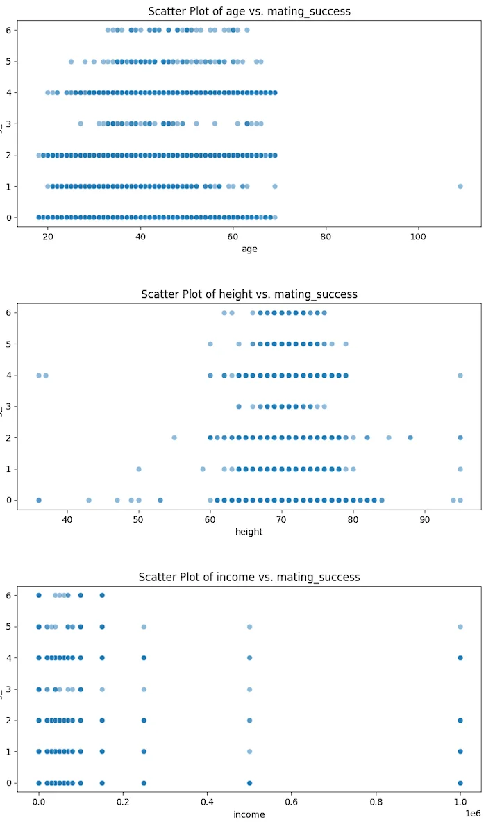
Mating success tends to increase with age, peaking in middle age.

This could be due to greater maturity, stability, or experience that may attract more partners.

There is a slight positive correlation between height and mating success.

Taller individuals may be perceived as more attractive due to societal preferences for height.

Higher-income shows a weak correlation with mating success.

Financial stability might contribute to higher attractiveness, but it's not the sole factor in mating success.

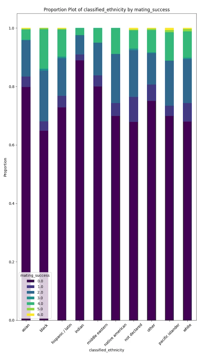
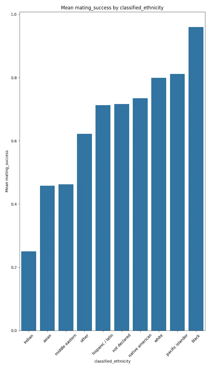
Ethnicities with significantly higher proportions of mating success in California are Whites, Pacific Islanders, and Blacks.

Ethnicities with significantly lower proportions of mating success in California are Indians, Middle Easterners, and Asians.

Cultural disparity could be one of the many driving forces for these results.

Also, different behaviours (between ethnicities), media, and politically driven depictions of ethnic groups could explain such results.

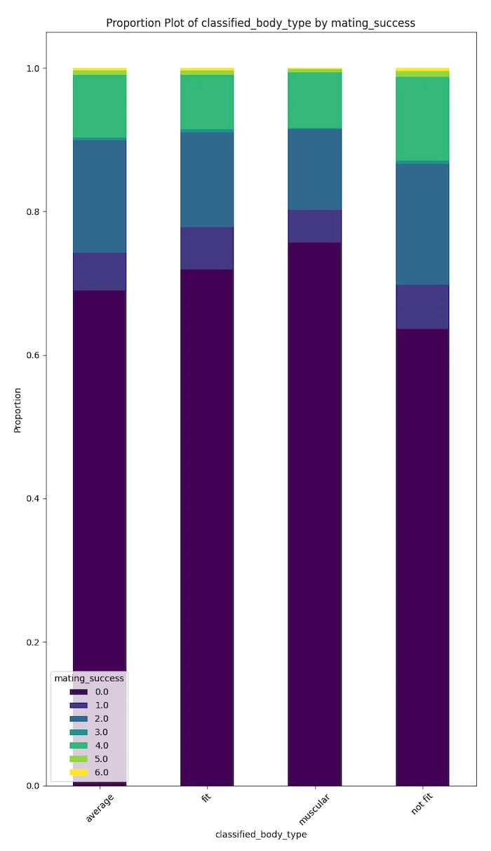
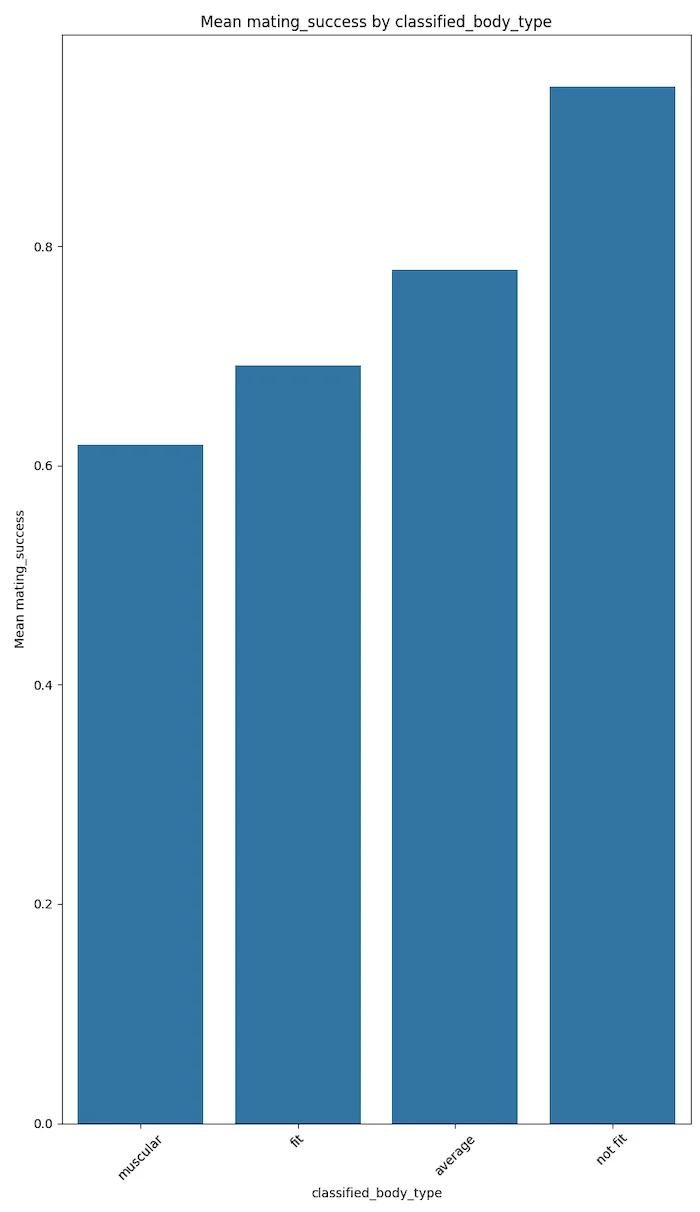
Body composition does not strongly affect having a 'partner' or 'kid.' However, bodies with 'dad bods' (not fit) have positive potential in terms of mating success.

We can suggest that muscular and fit body types are more positively correlated with hookup culture. However, this needs different data analyses to be confirmed.

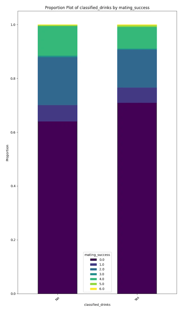
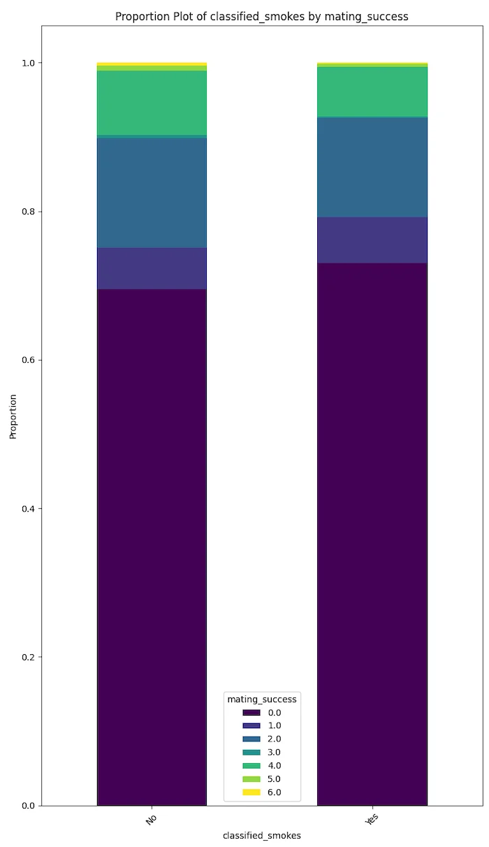
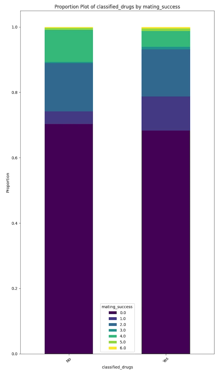
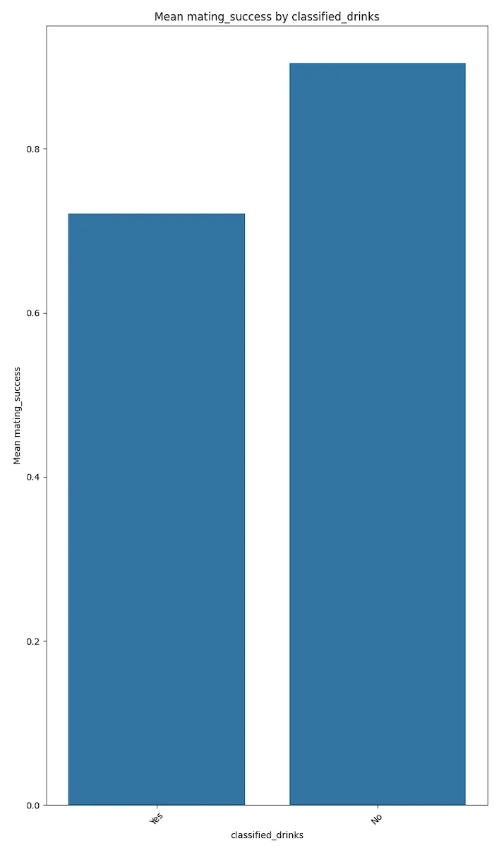
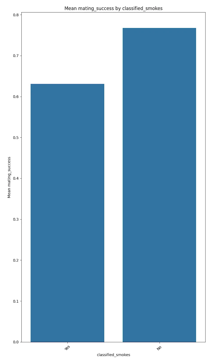
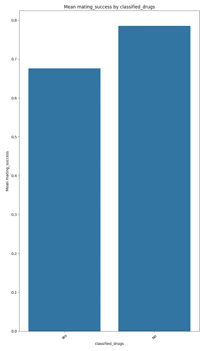
Degenerate behaviours like drinking, smoking and drug use seem to be negatively correlated with mating success.

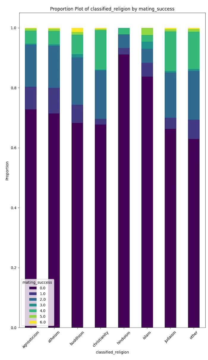
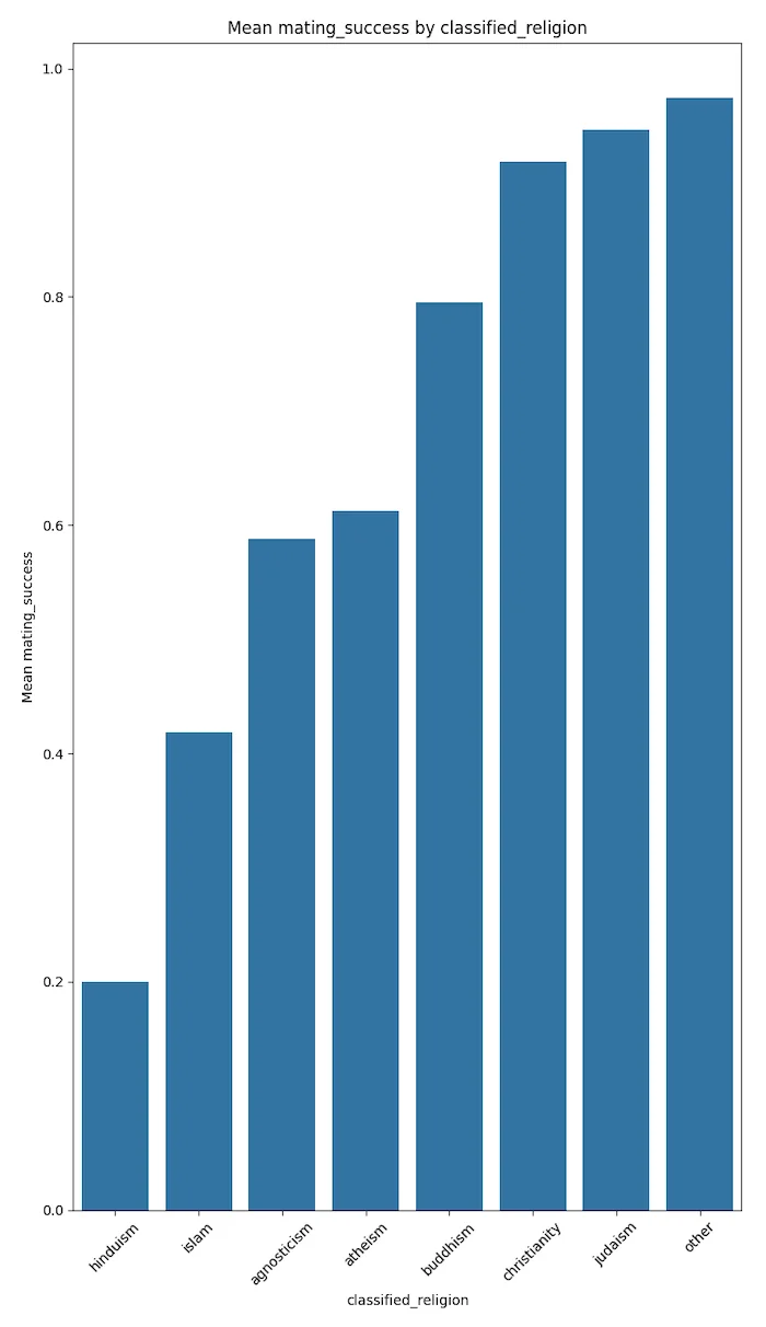
People adopting Hindu and Islamic spiritual beliefs seem to be the least able to secure long-term relations and progeny in California.

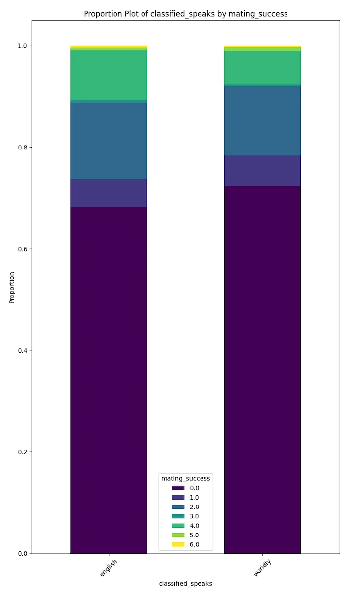
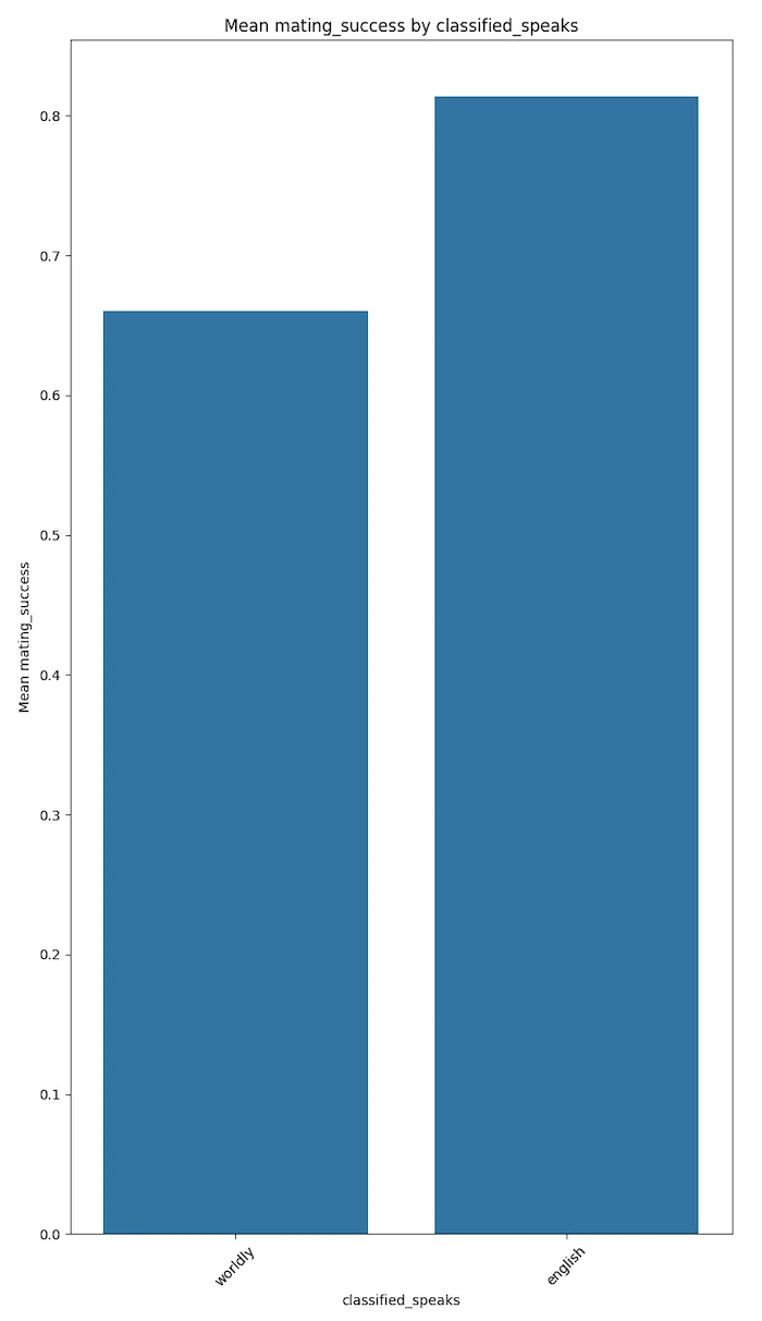
The plots below speak for themselves.

These results could trend to magnify if the votes were not self disclosed but were more factual. This conjecture needs to be proven with more factual data.

Links to other parts of the project

• OkCupid Dataset Analysis for Machine Learning
• Exploring OkCupid Dataset with Machine Learning: Predicting Mating Success for Straight Males
• Exploring OkCupid Dataset with Stratified Sampling
• OkCupid Dataset: Preparing the Data Before Learning Algorithms
• Comparing Model Performance: Linear Regression, Decision Tree, and Random Forest for Predicting Mating Success