Exploring OkCupid Dataset with Stratified Sampling

Challenges with Random Sampling and Feature Imbalance

In the preceding blog titled Exploring OkCupid Dataset with Machine Learning: Predicting Mating Success for Straight Males, we split the dataset to retrieve the test and train data using a random sampling method.

However, the random sampling method we used in the previous blog does not maintain the ratio of a specific feature in the dataset, which is a significant issue.

For example, if 60% of entries in our dataset have an ethnicity feature set to 'Middle Eastern,' we want that same proportion represented in the test set.

Otherwise, the sampling is skewed.

Exploring Possible Ethnicity Values for Classification

We will examine all the possible values that the features can take to facilitate the classification of our total dataset entries based on ethnicity.

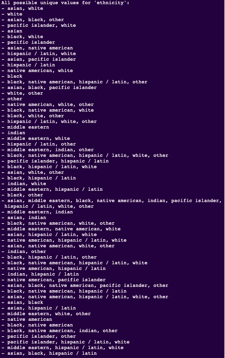
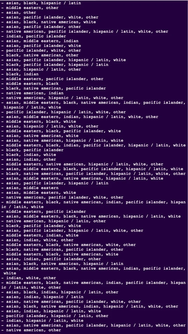
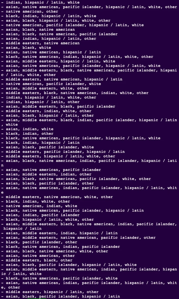
As you can see above, the ethnicity feature can take too many possible values, creating broader groups to reduce the number of possible categories.

Grouping Ethnicities into Strata for Machine Learning

In machine learning, each category is called a 'stratum '. Each stratum should have sufficient instances. Otherwise, the estimate of a stratum's importance may be biased by too little non-representative data.

We execute the code below to create a new column named classified_ethnicity and will follow the programming rules below to classify the entry into one specific ethnicity classification:

./chapter2/data2/data_manipulations2/step3.py

import os
import pandas as pd

# Define the path to the dataset folder
DATING_PATH = os.path.join("datasets", "dating")

# Function to load the dataset (male-only, straight)
def load_dating_data(dating_path=DATING_PATH):
    csv_path = os.path.join(dating_path, "male_straight_data_with_persistent_id.csv")
    return pd.read_csv(csv_path)

# Function to classify ethnicity
def classify_ethnicity(ethnicity):
    # Handle non-string, NaN, or empty string values
    if not isinstance(ethnicity, str) or pd.isna(ethnicity) or ethnicity.strip() == '':
        return 'not declared'
    
    # Split the ethnicity string by commas
    ethnicities = [eth.strip().lower() for eth in ethnicity.split(',')]
    
    # Classify based on the number of ethnicities
    if len(ethnicities) == 1:
        return ethnicities[0]
    elif len(ethnicities) == 2:
        return ethnicities[0]
    else:
        return 'other'

# Load the dataset
male_data = load_dating_data()

# Apply the ethnicity classification and add it as a new column
male_data['classified_ethnicity'] = male_data['ethnicity'].apply(classify_ethnicity)

# Save the updated dataset with the new column
output_path = os.path.join(DATING_PATH, "male_straight_data_with_persistant_id_classified_ethnicity.csv")
male_data.to_csv(output_path, index=False)

print(f"Dataset with classified ethnicity saved to: {output_path}")

Here is a snip of the data before and after classification:

Visualizing Classified Ethnicities

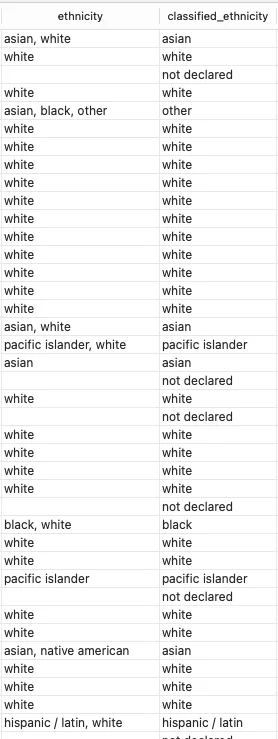
After the classification is established, we can proceed to plot the graph. This gives us an idea of the proportions of groups of people represented in our dataset .

We use the code below to generate the plots.

./chapter2/data2/plots/plot1.py

import pandas as pd
import matplotlib.pyplot as plt

# Load the dataset from the CSV file
file_path = "datasets/dating/male_straight_data_with_persistant_id_classified_ethnicity.csv"
data = pd.read_csv(file_path)

# Verify the data loaded correctly
print(data.head())

# Plot a histogram of the 'classified_ethnicity' column
plt.figure(figsize=(10, 6))  # Adjust the size of the plot
data['classified_ethnicity'].value_counts().plot(kind='bar', color='skyblue', edgecolor='black')

# Add titles and labels
plt.title('Distribution of Classified Ethnicities', fontsize=16)
plt.xlabel('Classified Ethnicity', fontsize=12)
plt.ylabel('Count', fontsize=12)

# Rotate x-axis labels for better readability
plt.xticks(rotation=45, ha='right')

# Display the plot
plt.show()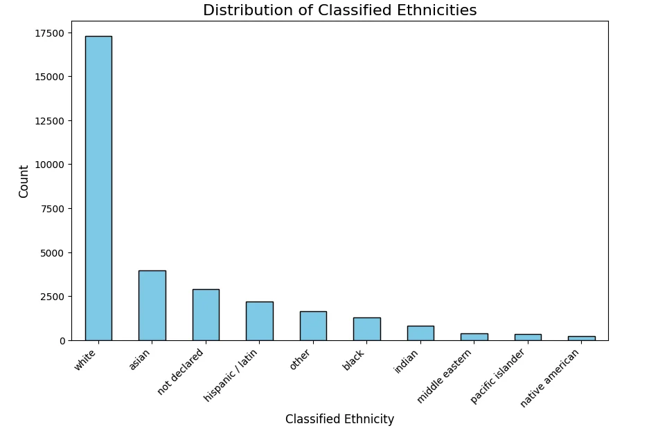

Performing a Stratified Split

We can now do a stratified split based on the classified ethnicity feature and maintain the same ratios in our test and training data:

We use Scikit-Learn's StratifiedShuffleSplit class:

./chapter2/data2/data_manipulations2/step4.py

from sklearn.model_selection import StratifiedShuffleSplit
import pandas as pd

# Load the dataset
file_path = "datasets/dating/male_straight_data_with_persistant_id_classified_ethnicity.csv"
dating_data = pd.read_csv(file_path)

# Verify the dating_data loaded correctly
print(dating_data.head())

# Initialize StratifiedShuffleSplit with one split and 20% test size
split = StratifiedShuffleSplit(n_splits=1, test_size=0.2, random_state=42)

# Perform stratified split based on 'classified_ethnicity'
for train_index, test_index in split.split(dating_data, dating_data['classified_ethnicity']):
    strat_train_set = dating_data.loc[train_index]
    strat_test_set = dating_data.loc[test_index]


# Save the persistent IDs to CSV files for future use
strat_train_set['persistent_id'].to_csv('datasets/dating/male_straight_data_with_persistant_id_classified_ethnicity_stratified_train_ids.csv', index=False)
strat_test_set['persistent_id'].to_csv('datasets/dating/male_straight_data_with_persistant_id_classified_ethnicity_stratified_test_ids.csv', index=False)

print("Train and test sets saved with persistent IDs.")

# Verify the size of the split datasets
print(f"Training set size: {len(strat_train_set)}")
print(f"Test set size: {len(strat_test_set)}")

# Optional: Check the distribution of classified ethnicities in train and test sets
print("Training set ethnicity distribution:")
print(strat_train_set['classified_ethnicity'].value_counts(normalize=True))

print("\nTest set ethnicity distribution:")
print(strat_test_set['classified_ethnicity'].value_counts(normalize=True))

# Save the train and test sets with proper names
train_file_path = "datasets/dating/male_straight_data_with_persistant_id_classified_ethnicity_stratified_train_set.csv"
test_file_path = "datasets/dating/male_straight_data_with_persistant_id_classified_ethnicity_stratified_test_set.csv"

strat_train_set.to_csv(train_file_path, index=False)
strat_test_set.to_csv(test_file_path, index=False)

# Check the overall distribution of classified ethnicities in the original dataset
print("Overall ethnicity distribution (entire dataset):")
print(dating_data['classified_ethnicity'].value_counts(normalize=True))

print(f"Training set saved to: {train_file_path}")
print(f"Test set saved to: {test_file_path}")

The image below shows the distributions of the total, train, and test datasets based on the classified_ethnicity feature.

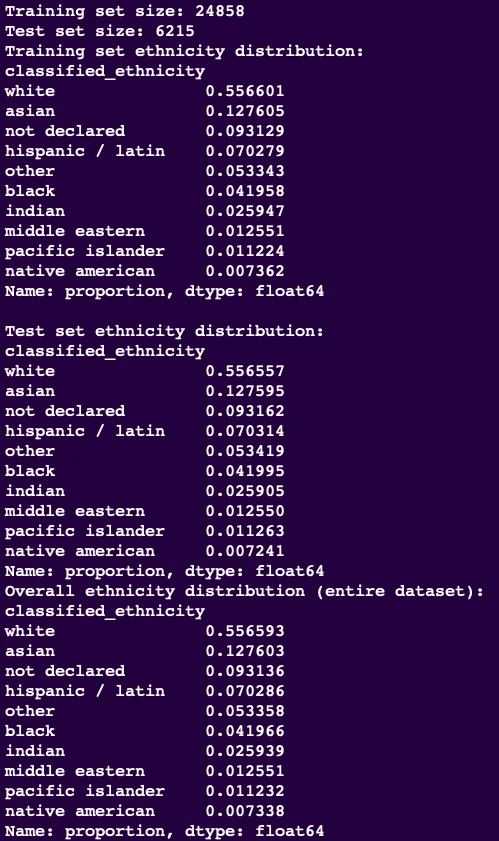
Notice the consistency of proportions across all total datasets and split test and train datasets.

Rebooting the Dataset After Deletions

If after a re-split, after some entries got deleted, we want to reboot the same entries in each test/train group, we can leverage the script below to do so:

./chapter2/data2/data_manipulations2/step5.py

import pandas as pd

# Load the updated dataset (after deletions or modifications)
file_path = "datasets/dating/male_straight_data_with_persistant_id_classified_ethnicity.csv"
updated_data = pd.read_csv(file_path)

# Load the saved train and test IDs
train_ids = pd.read_csv('train_ids.csv')['persistent_id']
test_ids = pd.read_csv('test_ids.csv')['persistent_id']

# Restore the original train and test sets using the persistent IDs
restored_train_set = updated_data[updated_data['persistent_id'].isin(train_ids)]
restored_test_set = updated_data[updated_data['persistent_id'].isin(test_ids)]

# Display the restored sets
print("Restored Training Set:")
print(restored_train_set)

print("\nRestored Test Set:")
print(restored_test_set)

Conclusion

We're ready to proceed with the classified ethnicity feature established and balanced through stratified sampling. In the next part of this series, we'll explore data visualization techniques to uncover patterns and insights hidden within the dataset.

Appendix

• Data Labels
• Yellow: Original data used for the split
• Red: After split IDs
• Gray: Test or Train Data

Links to other parts of the project

• OkCupid Dataset Analysis for Machine Learning
• Exploring OkCupid Dataset with Machine Learning: Predicting Mating Success for Straight Males
• Discover and Visualize the Data to Gain Insights on Feature vs Label Correlations: OkCupid Dataset
• OkCupid Dataset: Preparing the Data Before Learning Algorithms
• Comparing Model Performance: Linear Regression, Decision Tree, and Random Forest for Predicting Mating Success